Analysis of two mechanisms of telomere maintenance based on the theory of g-Networks and stochastic automata networks

Abstract

*

Background Telomeres, which are composed of repetitive nucleotide sequences at the end of chromosomes, behave as a division clock that measures replicative senescence. Under the normal physiological condition, telomeres shorten with each cell division, and cells use the telomere lengths to sense the number of divisions. Replicative senescence has been shown to occur at approximately 50–70 cell divisions, which is termed the Hayflick’s limit. However, in cancer cells telomere lengths are stabilized, thereby allowing continual cell replication by two known mechanisms: activation of telomerase and Alternative Lengthening of Telomeres (ALT). The connections between the two mechanisms are complicated and still poorly understood.

*

Results In this research, we propose that two different approaches, G-Networks and Stochastic Automata Networks, which are stochastic models motivated by queueing theory, are useful to identify a set of genes that play an important role in the state of interest and to infer their previously unknown correlation by obtaining both stationary and joint transient distributions of the given system. Our analysis using G-Network detects five statistically significant genes (CEBPA, FOXM1, E2F1, c-MYC, hTERT) with either mechanism, contrasted to normal cells. A new algorithm is introduced to show how the correlation between two genes of interest varies in the transient state according not only to each mechanism but also to each cell condition.

*

Conclusions This study expands our existing knowledge of genes associated with mechanisms of telomere maintenance and provides a platform to understand similarities and differences between telomerase and ALT in terms of the correlation between two genes in the system. This is particularly important because telomere dynamics plays a major role in many physiological and disease processes, including hematopoiesis.

Background

The introduction of Stochastic Automata Networks (SANs) [1] has led researchers to explore an efficient solution of finite multi-component Markov chains of potentially very high dimension. The main idea of the SAN formalism is to employ Kronecker algebra operations for generating the infinitesimal generator (also known as an intensity matrix or transition rate matrix) of a Markov chain in a product form in order to ease the problem of dimensionality and the complexity of the vector-matrix product [2, 3]. Specifically, a compact representation using tensor product and sums of matrices of the form, which is formally proved in [1]

$$\begin{array}{*{20}l} Q = \bigoplus_{i=1}^{N} L_{i} + \sum_{r = 1}^{R} \; \left(\; \bigotimes_{i=1}^{N} \; M_{r,i} + \bigotimes_{i=1}^{N} \; N_{r,i} \; \right), \end{array} $$

(1)

provides the transition rates of a time-continuous Markov chain of the type just described. Notation: N is the number of automata, R is the number of synchronizations, and L_i and M_r,i are matrices containing information about the local transitions and the effect of the synchronization r on the automaton i, respectively. N_r,i is the normalizing matrix of M_r,i, and ⊗ and ⊕ denote, respectively, the (generalized) tensor product and tensor sum [4]. Notation will be discussed in detail in the following section.

For a decade after SAN introduction, many outstanding analytical results have been proved. For example, Plateau and Stewart [5] proved in year 2000 that a product-form steady-state distribution for SANs without synchronizations exists, as long as some numerical conditions related to local balance are satisfied. Prior to that, Boujdaine et al. in 1997 [6] considered a special class of SAN having limited synchronization, and proved a sufficient condition for existence of stationary distribution, by applying properties of Kronecker sum. Note that classic queuing networks such as Jackson’s networks and G-Networks with positive and negative customers [7] fall under this special class.

Most analyses and applications of SANs focus on finding steady-state distribution of queuing system models. To our knowledge, correlation analysis in SANs is rarely examined, although correlation quantifies the degree of inter-relatedness of two automata. It contributes to the understanding of how the association of two automata changes with time according to the state of interest, with the behavior of other automata in the system simultaneously considered. In the current study, we first examine the exact-form of an infinitesimal generator for G-Networks with positive and negative customers. Then it is applied to a gene regulatory network (GRN) having five genes related to the onset of cancer in order to show the time-dependent dynamics of transition rates and correlation between two particular genes of interest. Throughout this paper, our analysis is based on time-continuous Markov chains, but we note that most results are valid in the time-discrete case provided complications such as periodicity are excluded.

Stochastic automata network

The SAN consists of a number of automata, which are correlated by synchronizing transitions. Each automaton has states and transitions. The state space of the system is the Cartesian product of the states of the automata [6]. There exist two types of transitions: local and synchronizing.

• 1. Transition in one automaton may initiate a new simultaneous transition in another automaton. Such transitions are collectively referred to as synchronizing transitions. In one synchronizing transition, two automata are paired. The first is called a master automaton; it affects the state of another automaton as its state changes. The second is called a slave automaton; it is affected by its master automaton [8].

• 2. In any given automaton, transitions not classified as synchronizing transitions are local transitions. Such transitions only change the state of one automaton.

In the SAN, two assumptions are made. First, the time to transition is exponentially distributed, and second, that a multidimensional Markov chain represents the SAN, although a particular automaton may not be Markovian itself. Then the (global) infinitesimal generator (the matrix of time derivatives at 0 of the transition probabilities), which reflects a change in transition probability from one state to another, is given by Eq. 1, with notation explained in Table1.

Table 1 Description of the notation in Eq. 1

Specifically, each matrix in Q is defined as follows:

• L_i is a local normalized transition rate matrix of automaton i; thus

  $$\begin{array}{*{20}l} L_{i}[m,n] \geq 0 \;\; \text{if} \;\; m \neq n \;\;\; \text{and} \;\;\; \sum_{n = 1}^{N} L_{i}[m,n] = 0 \end{array} $$

• For each synchronizing transition, for all i∈{1,2,⋯,N},M_r,i=I_K, where I_K is an identity matrix of size K, except for the case when r is two indices corresponding to master and slave automaton. Therefore

  $$ {{{}\begin{aligned} \bigotimes_{i=1}^{N} \; M_{r,i} & = I_{K} \otimes \cdots \otimes I_{K} \otimes \left(D_{r, msr(r)} - \bar{D}_{r, msr(r)} \right) \\ & \;\;\;\;\; \otimes I_{K} \otimes \cdots \otimes I_{K} \otimes E_{r, sl(r)} \otimes I_{K} \otimes \cdots \otimes I_{K} \end{aligned}}} $$

  where msr(r) and sl(r) are indices for master automaton and slave automaton, respectively, in the r^th synchronization. Here, D_r,msr(r) denotes the transition rate matrix due to the r^th synchronizing event on the master automaton, and $\bar {D}_{r, msr(r)}$ is its diagonal matrix. E_r,sl(r), the transition probability matrix, is the effect of the r^th synchronizing event on the automaton sl(r).

  $${{\begin{aligned} D_{r,msr(r)} [m, n] & \geq 0 \; \text{if} \; m \neq n \; & \text{and} \; & \sum_{n=1}^{N} D_{r,msr(r)} [m, n] & = 0 \;, \; \forall \; m \\ E_{r, sl(r)}[m,n] & \geq 0 \; \forall \; m, n & \text{and} \; & \sum_{n = 1}^{N} E_{r, sl(r)}[m,n] & = 1 \;, \forall \; m \end{aligned}}} $$

• A normalizing matrix $\bigotimes _{i=1}^{N} \; N_{i, r}$ is a (K^N×K^N)-dimensional diagonal matrix, whose the l^th diagonal element is the negative sum of the l^th row of $\bigotimes _{i=1}^{N} \; M_{r,i}$.

G-Networks with positive and negative customers

Gelenbe- or G-Networks [9], devised by Erol Gelenbe, are Markovian stochastic models grounded in queueing network theory [10]. They were extensively applied to study probability models of various objects [11–18]. However they are particularly appropriate to construct GRNs, as they introduce a novel notion called a ‘negative customer’, which can be biologically interpreted as a repression signal [19]. G-Networks model the number of positive customers, which is mRNA expression level biologically, in an automaton or a gene having an infinite state space. Positive and negative customers synchronously move from a master gene to a slave gene within the system with transition probabilities, $p_{msr(r), sl(r)}^{+}$ and $p_{msr(r), sl(r)}^{-}$, respectively. It implies that there are two types of the synchronizing transition. Note that the behavior of positive customers identical to that of positive customers in Jackson networks [20]. In contrast, negative customers function distinctively as follows: they are not accumulated and instantaneously leave a queue after the completion of their tasks. If a negative customer arrives at a non-empty queue, it destroys one current positive customer. However if the queue is empty, then the negative customer disappears without locally affecting the queue. Both types of customers arrive at the i^th gene from outside of the system at rates $\lambda _{i}^{+}$ and $\lambda _{i}^{-}$, respectively. It is assumed that service disciplines are the same for all queue [21], and the service times for each queue i are independent and identically exponentially distributed with rates μ_i∈(0,∞) for i=1,2,⋯,N. Figure 1 visually illustrates four activities of mRNA and/or protein molecules, and Table 2 suggests how the biological terms that refer to these activities can be identified with those used in G-Networks.

Fig. 1

Four activities for gene regulation in a G-network model

Table 2 Vocabulary and notation for application of G-Networks to Gene Regulatory Networks

G-Networks have an advantageous property of being analytically tractable because of the existence of product-form stationary distributions under the typical Markov Chain assumptions as shown in Eq. 2 [7, 22].

Let x={x₁,x₂,⋯,x_N} be the vector of non-negative integers representing the state of the network. Then the time-dependent vector, {x(t):t≥0}, is a continuous-time Markov chain, which satisfies the system of Chapman-Kolmogorov equations [23]. Element x_i(t),1≤i≤N, of vector x(t)=(x₁(t),x₂(t),⋯,x_N(t)), is the number of customers (or the mRNA expression level) of gene i at time t. It has been proved that the joint steady-state distribution π(x) of x(t), has the form of a product of stationary distributions of each queue,

$$\begin{array}{*{20}l} \pi \left(x \right) = \lim\limits_{t \rightarrow \infty} P \left(\boldsymbol{X}(t) = \boldsymbol{x} \right) = \prod_{i=1}^{N} \left(1 - q_{i} \right) \cdot q_{i}^{x_{i}} \end{array} $$

(2)

each satisfying the balance equation of the G-Networks [23–25], i.e.

$$\begin{array}{*{20}l} q_{i} \,=\, \lim\limits_{t \rightarrow \infty} P \left(x_{i}(t) > 0 \right) \,=\, \frac{\lambda_{i}^{+} + \sum_{j=1}^{N} q_{j} \cdot \mu_{j} \cdot p_{{ji}}^{+}}{\mu_{i} + \lambda_{i}^{-} + \sum_{j=1}^{N} q_{j} \cdot \mu_{j} \cdot p_{{ji}}^{-}} > 0, \end{array} $$

(3)

for i=1,2,⋯,N. It implies that the stationary probability for each positive recurrent state is expressed in the terms of a product of functions depending solely on the state of a single queue.

According to [8], matrices constituting the global infinitesimal generator Q are defined as follows in the terms of customer-related rates:

$${{\begin{aligned} L_{i} & = \lambda_{i}^{+} \left(Upp - I_{K}^{0} \right) + \mu_{i} d_{i} \left(Low-I_{1}^{0} \right) + \lambda_{i}^{-} \left(Low - I_{1}^{0} \right), \forall \; i \in \mathbb{N} \\ D_{r, msr(r)} & = \left\{\begin{array}{ll} & \mu_{i} \cdot \; p_{msr(r), sl(r)}^{+} \cdot \left(Low-I_{1}^{0} \right) \\ & \text{, if a customer leaves a master automaton} \\ & \text{and moves to a slave automaton as a} {positive} \text{ customer} \\ & \mu_{i} \cdot \; p_{msr(r), sl(r)}^{-} \cdot \left(Low-I_{1}^{0} \right) \\ & \text{, if a customer leaves a master automaton} \\ & \text{and moves to a slave automaton an as a } {negative} \text{ customer} \end{array}\right. \\ E_{r, sl(r)} & = \left\{\begin{array}{ll} \; Upp & \text{, if a } {positive} \text{ customer arrives at a slave automaton} \; sl(r) \\ \; Low & \text{, if a } {negative} \text{ customer arrives at a slave automaton} \; sl(r) \end{array}\right. \\ \bigotimes_{i=1}^{N} \; N_{r,i} & = \left\{\begin{array}{ll} I_{K} \otimes \cdots \otimes I_{K} \otimes \bar{D}_{r, msr(r)} \otimes I_{K} \otimes \cdots \otimes I_{K} \otimes I_{K}^{0} \otimes I_{K} \otimes \cdots \otimes I_{K} \\ \;\;\;\;\;\;\;\;\;\;\;\;\;\;\;\; \text{, if a slave automaton receives a positive customer} \\ I_{K} \otimes \cdots \otimes I_{K} \otimes \bar{D}_{r, msr(r)} \otimes I_{K} \otimes \cdots \otimes I_{K} \otimes I_{1}^{0} \otimes I_{K} \otimes \cdots \otimes I_{K} \\ \;\;\;\;\;\;\;\;\;\;\;\;\;\;\;\; \text{, if a slave automaton receives a negative customer} \end{array}\right. \end{aligned}}} $$

where

• I : Identity matrix

• Upp : Matrix with entries 0 except the main upper diagonal which is 1

• Low : Matrix with entries 0 except the main lower diagonal which is 1

• $I_{1}^{0}$ : Identity matrix except the first diagonal element which is 0

• $I_{K}^{0}$: Identity matrix except the K^th diagonal element which is 0

Results

This section consists of two parts. The first part shows the mathematical result that derives the correlation between two genes utilizing Kronecker algebra. The second part contains the biological results based on the application of the mathematical result to the gene regulatory network associated with telomere biology.

Mathematical result: derivation of joint transient distribution of two automata

If Q is the infinitesimal generator and P(t) is the transition probability matrix of a finite Markov chain, we can derive a set of differential equations called Kolmogorov’s forward equations, in the form of P^′(t)=P(t)·Q. Solution of the forward equation is given in this case by the power series expansion that converges for any square matrix Q:

$$\begin{array}{*{20}l} P(t) = e^{Qt} = \sum_{n=0}^{\infty} \frac{\left(Qt \right)^{n}}{n!}. \end{array} $$

(4)

The resulting (1×K^N)-dimensional time-dependent state probability vector at time t has the form

$$\begin{array}{*{20}l} \pi(t) =\pi(0) \cdot e^{Qt} \end{array} $$

(5)

where π(t) is a state probability vector at time t [26]. In order to find a joint state probability vector π_i,j(t) of two automata, say i and j, we introduce two matrices C_i,j and $C^{*}_{i,j}$, which are (K^N×K²)- and (K²×K^N)-dimensional, respectively. After several steps of calculation, we obtain

$$\begin{array}{*{20}l} \pi_{i,j}(t) & = \underbrace{\pi(t)}_{\text{\(1 \times K^{N}\)}} \cdot \underbrace{C_{i,j}}_{\text{\(K^{N} \times K^{2}\)}} \\ & \Rightarrow \; C^{*}_{i,j} \cdot C_{i,j} \cdot e^{Q_{i,j} \; t} = C^{*}_{i,j} \cdot e^{Q \; t} \cdot C_{i,j} \;, \end{array} $$

(6)

where, for all i≠j, i,j=1,2,⋯,N, C_i,j and $C^{*}_{i,j}$ are defined by

$${\begin{aligned} \underbrace{C_{i,j}}_{\text{\(K^{N} \times K^{2}\)}} = \bigotimes_{n=1}^{N} \; U_{i,j,n} \;\;\; &, \;\;\; U_{i,j,n} = \left\{\begin{array}{ll} \;\; I_{K} \;\; & \; \text{, if} \; n = i \; \text{or} \; n = j \\ \;\; 1_{K} \;\; & \; \text{, if} \; n \neq i \; \text{and} \; n \neq j \end{array}\right. \\ \underbrace{C^{*}_{i,j}}_{\text{\(K^{2} \times K^{N}\)}} = \bigotimes_{n=1}^{N} \; V_{i,j,n} \;\;\; &, \;\;\; V_{i,j,n} = \left\{\begin{array}{ll} \;\; I_{K} \;\; & \; \text{, if} \; n = i \; \text{or} \; n = j \\ \;\; 1^{T}_{K} \;\; & \; \text{, if} \; n \neq i \; \text{and} \; n \neq j \;\;\;. \end{array}\right. \end{aligned}} $$

Note that the (1×K)-dimensional matrix $1_{K}^{T} = \left [\begin {array}{llll} 1 & 1 & \cdots & 1 \end {array}\right ]$ indicates the matrix transpose of 1_K. This results in

$$\begin{array}{*{20}l} C^{*}_{i,j} \cdot C_{i,j} = \left(\bigotimes_{n=1}^{N} \; V_{i,j,n} \right) \cdot \left(\bigotimes_{n=1}^{N} \; U_{i,j,n} \right) = K^{N-2} \cdot I_{K^{2}} \;\;, \end{array} $$

(7)

where

$$\begin{array}{*{20}l} V_{i,j,n} \cdot U_{i,j,n} = \left\{\begin{array}{ll} I_{K} \;\;\; & \;\;\; \text{, if} \; n = i \; \text{or} \; n = j \\ K \;\; (\text{a scalar}) \;\;\; & \;\;\; \text{, if} \; n \neq i \; \text{and} \; n \neq j \;\;. \end{array}\right. \end{array} $$

Therefore Eq. 6 finally becomes

$$\begin{array}{*{20}l} e^{Q_{i,j} \cdot t} = \frac{1}{K^{N-2}} \cdot C^{*}_{i,j} \cdot e^{Q \; t} \cdot C_{i,j} \;\;. \end{array} $$

(8)

Equation 8 implies that a time-dependent joint state probability vector π_i,j(t) can be easily calculated, once the infinitesimal generator, Q, of the entire system is obtained.

$$\begin{array}{*{20}l} {}& \pi_{i,j}(t) \; = \; \pi_{i,j}(0) \cdot e^{Q_{i,j} \cdot t} \\ & = \; \frac{1}{K^{N-2}} \cdot \pi_{i,j}(0) \cdot C^{*}_{i,j} \cdot e^{Q t} \cdot C_{i,j} \\ & = \; \left\{ p_{0, 0}(t), \; p_{0, 1}(t), \; p_{0, 2}(t) \cdots,\right. \\& \;\left. p_{K-1, K-2}(t), \; p_{K-1, K-1}(t) \right\} \end{array} $$

(9)

We can then form a (K×K)-dimensional table that describes the joint probabilities for each time point t. Based upon it, the association between two genes for all t is evaluated using the Pearson product-moment correlation coefficient [27]. It implies the correlation of a pair of genes in the regulatory system varies by each time (each generation of cells) as shown in Fig. 2.

Fig. 2

The correlation of a pair of genes. The correlation of a pair of genes can be either positive (green solid line) or negative (red dashed line). The thicker line represents the stronger correlation of two connected genes, while the thinner line indicates the weaker correlation of them

Application to the gene regulatory networks

GRNs and parameters from g-Networks

In this research, we use a GRN provided in Fig. 3. It consists of 5 statistically significant genes associated with telomere maintenance, which are discovered by (modified) Abnormal Pathway Detection Algorithm (APDA) based on G-Networks [18]. (See Methods for detailed information on the modification). We explore the correlation between a pair of genes, e.g., CEBPA and hTERT, which is not apparent from Fig. 3. On the biology side, Kirwan et al. in 2009 [28] reported that mutations in hTERT within 4 of 20 families were identified in familial acute myeloid leukemia (AML). It is known that the mutation of CEBPA is one of the important factors in AML and its prognosis [29]. However the direct relationship between CEBPA and AML is still not satisfactorily understood. The joint state probability vector of two genes, which can be calculated from Eq. 9, is expected to show the flow of probabilities for the K²–tuples of mRNA expression levels at each fixed time t, and thereby illustrates the relationship between any two genes.

Fig. 3

A network with 5 automata (genes) and 7 synchronizing transitions

In this case, the number of automata is equal to N=5, while the number of synchronizing events is equal to R=7. We limit the number of gene expression levels to K=7 for two reasons. The first is that, because the data are normalized, there are few genes with a mRNA expression level of 7 or higher. Furthermore, the memory limitations enforce it. In this paper, we assume that pairs of genes are highly positively correlated at the initial time point; that is

$$\begin{array}{*{20}l} p_{{ij}}(0) = {\left[\begin{array}{lllllll} \frac{5}{47} & \frac{1}{47} & 0 & 0 & 0 & 0 & 0 \\ \frac{1}{47} & \frac{5}{47} & \frac{1}{47} & 0 & 0 & 0 & 0 \\ 0 & \frac{1}{47} & \frac{5}{47} & \frac{1}{47} & 0 & 0 & 0\\ 0 & 0 & \frac{1}{47} & \frac{5}{47} & \frac{1}{47} & 0 & 0 \\ 0 & 0 & 0 & \frac{1}{47} & \frac{5}{47} & \frac{1}{47} & 0 \\ 0 & 0 & 0 & 0 & \frac{1}{47} & \frac{5}{47} & \frac{1}{47} \\ 0 & 0 & 0 & 0 & 0 & \frac{1}{47} & \frac{5}{47} \\ \end{array}\right]} \end{array} $$

Note that this matrix needs to be transformed into a (1×K²)-dimensional joint state probability vector as π_ij(t) in Eq. 9. Tables 3 and 4 exhibit the values of parameters that are required to build the infinitesimal generator Q. They are estimated and optimized according to the APDA [18] based on G-Networks. Specifically, values in Table 3 allow to calculate a joint probability vector π_i,j(t), under the normal condition, with the Table 4 contains information for malignant (ALT or active telomerase) cells. The three families of parameters, $\lambda _{i}^{+}, \lambda _{i}^{-}$ and μ_i for all i, are identical for both normal and ALT cells, while transition probabilities, $p_{{ij}}^{+}, p_{{ij}}^{-}$ and d_i, are different between the cell types. Transition probabilities are deciding factors in correlation coefficients based on Eq. 9 and the rates of convergence to stationarity in G-Networks.

Table 3 Values of the parameters needed to determine the infinitesimal generator (Q) using 4 normal cell lines, where $d_{i} = 1- \sum _{j=1}^{N} \left (p_{{ij}}^{+} + p_{{ij}}^{-}\right)$

Table 4 Values of the parameters that are needed to determine the infinitesimal generator (Q) using 18 ALT cell lines

Simulation study using estimated parameters

Estimated and/or assumed values of the parameters listed in Tables 3 and 4 determine the infinitesimal generator, Q, and the steady-state distribution of each gene. Developed on the global balance equation of G-Networks [23] and the exponentially-distributed holding times of Markov chains [30], the empirical cumulative density function (ECDF) was exploited to confirm that parameter estimation via the APDA is appropriate aligning with the theory of G-Networks. We compare the ECDF of simulated data utilizing values in Tables 3 and 4 and the theoretical cumulative density function (CDF) based on q_i in Eq. 3. The algorithm for the simulation is explained in detail in Methods.

The ECDF, usually denoted by $\hat {F}_{n} (x)$, is associated with cumulative frequency of observations (empirical sampled data). It is a non-parametric estimator of the underlying CDF of a random variable of interest and is formally defined as follows:

$$\begin{array}{*{20}l} \hat{F}_{n} (x) = \hat{P}_{n} \left(X \leq x \right) = \frac{1}{n} \cdot \sum_{i=1}^{n} \; \mathbbm{1}_{\left[ x_{i} \leq x \right]} \;\;, \end{array} $$

where $\mathbb{1}_{\left [ \cdot \right ]}$ is an indicator function. That is, the ECDF is a step function that increases by $\frac {1}{n}$ at each datum. The stationary probability distribution of each gene in G-Networks is in the geometric product-form as stated in Eq. 2, which results in the following tail of the theoretical CDF, T(x_i):

$$\begin{array}{*{20}l} T \left(x_{i} \right) = 1 - F \left(x_{i} \right) = 1 - \left(1 - q_{i}^{x_{i} + 1} \right) = q_{i}^{x_{i} + 1} \;\;. \end{array} $$

(10)

Figure 4 (and Fig. 9) illustrates how the ECDF of hTERT utilizing estimated/assumed values of the parameters (Tables 3 and 4) converges to the theoretical CDF regardless of cell types. Similar patterns are obtained for all 5 statistically significant genes in this research.

Fig. 4

ECDF plots of hTERT under the normal condition (top) and ALT (malignant) condition (bottom). Orange and green straight and thick lines represent theoretical (logarithmically transformed) CDF of normal and ALT conditions, respectively. Purple, blue (thin) and red (thick) lines serve as the logarithmically transformed ECDF of hTERT after 10 steps, 100 steps and 500 steps, respectively

Correlation between a pair of genes

We discuss the similarities or differences in the correlation of two genes between normal and malignant cells with either active telomerase or ALT. Figure 5 based on Eq. 9 illustrates the following:

• First, Fig. 5 demonstrates the change of correlation between a pair of genes in the given system over time in normal cells and ALT (malignant) cells. We can then infer both the trend of correlation between a pair of genes and the speed to the transient state, i.e., before it reaches a steady state. Due to the product-form stationary probability distribution of network state in the theory of G-Networks, the correlation coefficient becomes 0 when the system becomes stationary [31]. Assuming that the pair of genes are positively correlated at time 0, the positive correlation persists over time in both types of cells (normal and ALT) and practically reaches 0 (the steady state) approximately at t=0.8. As shown in the figure, the patterns of correlation between each pair of genes do not noticeably differ among the types of cells (normal or malignant with either ALT or active telomerase shown), although they are dissimilar from one pair to another within the same type of cells. For example, the correlation between CEBPA and FOXM1 in a transient state is stronger than that of c-Myc and hTERT, and it reaches a steady state more slowly in all cell types.

  Fig. 5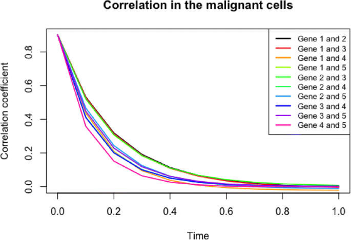

  

  Trend of correlation between each pair of genes in the system over time in ALT (malignant) cells. The general relationship of two genes in the system is similar regardless of the mechanism by which telomeres maintain their sufficient lengths. However, within the same condition of cells, the magnitude of correlation and the speed to the steady state vary by interactions

  Fig. 6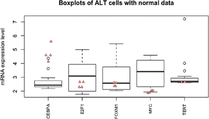

  

  A box plot displaying the five number summary of the five significant genes in ALT cells. Red triangle dots represent the mRNA expression levels of the corresponding gene in 4 normal cells

• Second, Eq. 9 uncovers the interactions between (1) CEBPA and hTERT, (2) FOXM1 and hTERT and (3) FOXM1 and E2F1, which are unknown in Fig. 3. The pattern in Fig. 5, which is analogous to Fig. 7, delineates that the relationship of the three pairs of genes is similar regardless of the mechanisms by which telomeres maintain their sufficient lengths. However, within the same condition of cells, the magnitude of correlation and the speed to the steady state vary by interactions. It is supported by the interaction of CEBPA and hTERT, which is relatively weaker than that of other pairs, even though its trend over time is indistinguishable by the cell types.

  Fig. 7

  

  Trend of correlation between a pair of genes in the system over time in (top) normal cells and (bottom) in malignant cells from 16 telomerase-positive cell lines

Note that if we conversely assume that a pair of genes are highly negatively correlated at the initial time point, then the negative correlation prevails over time as shown in Fig. 8.

Fig. 8

Trend of correlation between a pair of genes in the system over time in normal cells with the assumption that a pair of genes are initially negatively correlated

Fig. 9

ECDF plots of E2F1 under the normal condition (top) and ALT (malignant) condition (bottom). Orange and green straight and thick lines represent theoretical (logarithmically transformed) CDF of normal and ALT conditions, respectively. Top: Orange, blue, purple, red (thick) lines serves as the logarithmically transformed ECDF of E2F1 after 10 steps, 100 steps, 300 steps and 500 steps, respectively. Bottom: Orange, blue, purple, red (thick) lines serves as the logarithmically transformed ECDF of E2F1 after 10 steps, 100 steps, 500 steps and 1000 steps, respectively

Discussion

One important advantage of using mathematical modeling to understand dynamics of a biological system is that the model can be a cost-effective and time-saving supplement or even a substitute for laboratory experiments in which patterns of the system are delicate and complex. Especially the stochastic approach is useful to quantify the role of fluctuations in the behavior of the system of interest. In this paper, we propose that a stochastic paradigm involving G-Networks and Stochastic Automata Networks both stemming from queuing theory, can contribute to the analysis of similarities and differences between telomerase activation and ALT using genes related to telomere maintenance. However, there are the following two caveats.

• First, correlation coefficient, whose sign relies upon the initial joint state probability vector π_ij(0) in our example, evaluates the strength of the evidence for a relationship of two genes but does not determine causal relationships. In other words, even if a positive correlation between CEBPA and hTERT in ALT cells is revealed, it is not known which gene activates another one.

• Second, the dimension of the infinitesimal generator, Q, which is a function of tensor products, can be enormously large, with the corresponding matrix being sparse depending on the number of states of each queue. The state space used in this research is relatively small. Computations in larger dimensions can be made practical by using Compressed Sparse Row and a number of methods for the approximation of the matrix exponential [32] such as Krylov-type techniques.

Conclusion

In spite of the caveats discussed in the previous section, the APDA based on G-Networks initially introduced in [18] can suggest a set of statistically significant genes (CEBPA, FOXM1, E2F1, c-MYC, hTERT) in cells with either telomerase or ALT compared to normal cells from preexisting GRNs. We further confirmed that the APDA satisfactorily estimates the parameters, which decide the rates of convergence to stationarity as the ECDF of the simulated data using the estimated parameters approaches to theoretical CDF using q_{i∈{1,2,⋯,N}} as time progresses. Further, our correlation analysis based on SANs helps to infer the link between genes in various conditions that has not yet been discovered through experiments. We prove that our mathematical expression (Eq. 9) allows analytically calculating the correlation coefficients between any pair of genes in the given system at every time point and compare them in various types of cells for an order relation. Specifically in our example, the trend of correlation among genes in the system is not influenced by the mechanism (telomerase vs. ALT) by which telomeres maintain their sufficient lengths, even though the trend differs from one pair to another within the same type of cells. To conclude, this study provides a platform to detect significant genes and infer the previously unknown connection among them by applying modeling techniques borrowed from queueing theory. This is particularly important because telomere dynamics plays a major role in many physiological and disease processes, including hematopoiesis.

Methods

Detailed proof of Eq. 9

If Q is the infinitesimal generator and P(t) is the transition probability matrix of a finite Markov chain, we can derive a set of differential equations called Kolmogorov’s forward equations, in the form of P^′(t)=P(t)·Q

$$\begin{array}{*{20}l} \frac{d}{dt} P(t) \equiv P^{\prime}(t) = P(t) \cdot Q \;. \end{array} $$

P(0) initial condition is P(0)=I, where I is an identity matrix having the same dimension as Q [33], consistent with

$$\begin{array}{*{20}l} p_{{ij}}(0) = \left\{\begin{array}{ll} P \left(\; X(0) = i \; | \; X(0) = i \; \right) = 1 \;\;\; &\text{, if} \; i = j \\ P \left(\; X(0) = j \; | \; X(0) = i \; \right) = 0 \;\;\; &\text{, if} \; i \neq j \end{array}\right. \end{array} $$

Solution of the forward equation for finite Markov chains is given by the power series expansion that always converges for any square matrix Q:

$$\begin{array}{*{20}l} P(t) & = e^{Qt} && = \sum_{n=0}^{\infty} \frac{\left(Qt \right)^{n}}{n!} \\ & && = I + Qt + \frac{\left(Qt \right)^{2}}{2!} + \frac{\left(Qt \right)^{3}}{3!} + \frac{\left(Qt \right)^{4}}{4!} \cdots \\ & && \approx I + Qt + \frac{\left(Qt \right)^{2}}{2!} + \frac{\left(Qt \right)^{3}}{3!} + \|H(t)\|. \end{array} $$

(11)

where ||·|| denotes l₁-norm, and H(t) is is a linear operator with || H(t) ||=o(t), as t→0. When the infinitesimal generator, Q, is irreducible, its transition probability matrix, P(t) defined in Eq. 11, is strictly positive for each time t>0. It signifies that as the trajectory length N approaches to the limit, at least one transition between any pair of states will almost surely happen without regard to the sparsity of Q [34]. Note that 0=π·Q are a set of |S| linear equations, which is usually used to detect the stationary distribution π, if such one exists [26].

A formal solution to the time dependent state probability vector is defined as

$$\begin{array}{*{20}l} \pi(t) = \underbrace{\pi(0)}_{\text{\(1 \times K^{N} \)}} \cdot \underbrace{e^{Qt}}_{\text{\(K^{N} \times K^{N} \)}} \end{array} $$

(12)

where π(t) is a state probability vector at time t [35, 36]. In order to find a joint state probability vector π_i,j(t) of two automata, say i and j, we introduce two matrices called C_i,j and $C^{*}_{i,j}$, which are (K^N×K²)- and (K²×K^N)-dimensional matrices, respectively. Then based on Eq. 12, we achieve

$$\begin{array}{*{20}l} \begin{aligned} & &\pi_{i,j}(t) & = \underbrace{\pi(t)}_{\text{\(1 \times K^{N}\)}} \cdot \underbrace{C_{i,j}}_{\text{\(K^{N} \times K^{2}\)}} \\ & \Rightarrow \;\;\; & \pi_{i;j}(0) \cdot e^{Q_{i,j} \; t} & = \pi(0) \cdot e^{Q \; t} \cdot C_{i,j} \\ & \Rightarrow \;\; & \pi(0) \cdot C_{i,j} \cdot e^{Q_{i,j} \; t} & = \pi(0) \cdot e^{Q \; t} \cdot C_{i,j} \\ & \Rightarrow \;\; & C_{i,j} \cdot e^{Q_{i,j} \; t} & = e^{Q \; t} \cdot C_{i,j} \\ & \Rightarrow \;\; & C^{*}_{i,j} \cdot C_{i,j} \cdot e^{Q_{i,j} \; t} & = C^{*}_{i,j} \cdot e^{Q \; t} \cdot C_{i,j} \end{aligned} \end{array} $$

(13)

Here, C_i,j and $C^{*}_{i,j}$ are defined as follows respectively:

$${{\begin{aligned} \underbrace{C_{i,j}}_{\text{\(K^{N} \times K^{2}\)}} = \bigotimes_{n=1}^{N} \; U_{i,j,n} \;\;\;, \; \forall \; i \neq j \;, \; i = 1, 2, \cdots, N \;, \; j = 1, 2, \cdots, N \end{aligned}}} $$

where

$$\begin{array}{*{20}l} U_{i,j,n} = \left\{\begin{array}{ll} \;\; I_{K} \;\;\; & \;\;\; \text{, if} \; n = i \; \text{or} \; n = j \\ \;\; 1_{K} \;\;\; & \;\;\; \text{, if} \; n \neq i \; \text{and} \; n \neq j \end{array}\right. \end{array} $$

and

$${{\begin{aligned} \underbrace{C^{*}_{i,j}}_{\text{\(K^{2} \times K^{N}\)}} = \bigotimes_{n=1}^{N} \; V_{i,j,n} \;\;\;, \; \forall \; i \neq j \;, \; i = 1, 2, \cdots, N \;, \; j = 1, 2, \cdots, N \end{aligned}}} $$

where

$$\begin{array}{*{20}l} V_{i,j,n} = \left\{\begin{array}{ll} \;\; I_{K} \;\;\; & \;\;\; \text{, if} \; n = i \; \text{or} \; n = j \\ \;\; 1^{T}_{K} \;\;\; & \;\;\; \text{, if} \; n \neq i \; \text{and} \; n \neq j \;\;\;. \end{array}\right. \end{array} $$

Note that $1_{K}^{T}$ indicates the matrix transpose of 1_K, and we have

$$\begin{array}{*{20}l} \underbrace{1_{K}}_{\text{\(K \times 1\)}} & = \left[\begin{array}{l} 1 \\ 1 \\ \vdots \\ 1 \end{array}\right] \;\;\;\;\; \text{and} \;\;\;\;\; \underbrace{1_{K}^{T}}_{\text{\(1 \times K\)}}= \begin{bmatrix} 1 & 1 & \cdots & 1 \end{bmatrix}. \end{array} $$

This results in

$$\begin{array}{*{20}l} C^{*}_{i,j} \cdot C_{i,j} & = \left(\bigotimes_{n=1}^{N} \; V_{i,j,n} \right) \cdot \left(\bigotimes_{n=1}^{N} \; U_{i,j,n} \right) \\ & = \bigotimes_{n=1}^{N} \; V_{i,j,n} \cdot U_{i,j,n} \\ & = K^{N-2} \cdot I_{K^{2}} \end{array} $$

where

$$\begin{array}{*{20}l} V_{i,j,n} \cdot U_{i,j,n} = \left\{\begin{array}{ll} I_{K} \;\;\; & \;\;\; \text{, if} \; n = i \; \text{or} \; n = j \\ K \;\; (\text{a scalar}) \;\;\; & \;\;\; \text{, if} \; n \neq i \; \text{and} \; n \neq j \end{array}\right. \end{array} $$

Therefore Eq. 13 finally becomes

$$\begin{array}{*{20}l} \begin{aligned} & K^{N-2} \cdot I_{K^{2}} \cdot e^{Q_{i,j} \cdot t} && = C^{*}_{i,j} \cdot e^{Q \; t} \cdot C_{i,j} \\ \Rightarrow \;\;\; & e^{Q_{i,j} \cdot t} && = \frac{1}{K^{N-2}} \cdot C^{*}_{i,j} \cdot e^{Q \; t} \cdot C_{i,j} \end{aligned} \end{array} $$

(14)

Equation 14 implies that a time-dependent joint state probability vector π_i,j(t) can be easily calculated, once the (global) infinitesimal generator of the entire system is obtained.

$$\begin{array}{*{20}l} \pi_{i,j}(t) & \; = \; \underbrace{\pi_{i,j}(0)}_{\text{\(1 \times K^{2}\)}} \cdot \underbrace{e^{Q_{i,j} \cdot t}}_{\text{\(K^{2} \times K^{2}\)}} \; = \; \frac{1}{K^{N-2}} \cdot \pi_{i,j}(0) \cdot C^{*}_{i,j} \cdot e^{Q t} \cdot C_{i,j} \end{array} $$

(15)

Once π_i,j(t) of two genes is obtained, we then can form a (K×K)-dimensional contingency table that describes the joint probability for each time point t. Based upon it, the association between two genes for all t is evaluated using the Pearson product-moment correlation coefficient.

Application to telomere maintenance

Data description

Gene expression data (GSE14533) were obtained from the National Center for Biotechnology Information Gene Expression Omnibus (http://0-www-ncbi-nlm-nih-gov.brum.beds.ac.uk/geo/). Data includes expression gene levels of 3 types of cells: 18 ALT cell lines, 16 telomerase-positive cell lines and 4 normal (fibroblast) cell lines. Initially, the gene expression levels of 29 genes (hTERT, CRY2, FOXM1, c-MYC, SOCS1, AHNAK, HDAC5, TK1, S100A4, LMO4, PRKD1, PER2, PRKCA, CEBPA, E2F1, RBPJ, TOMM20, AIP, EHD1, TGOLN2, TTC17, LAMP2, ATP5D, ADGRL1, LASP1, RPRD1A, HNRNPA3, KAT2A, STK24) were extracted from the data according to [37]. However, only 5 significant genes (CEBPA, E2F1, FOXM1, c-MYC, hTERT) (connected to statistically significant edges) in either telomerase-positive or ALT cells compared to the normal cells, discovered by APDA based on G-Networks [18], have been included in this research. Note that the data were first normalized to the 50^th percentile to guarantee the identical medians across all samples. Then they were normalized again and scaled with mean 3 and variance 1 [18, 38]. Table 5 and Fig. 6 outline the data in detail.

Table 5 Mean mRNA expression levels (normalized and scaled) of genes in normal and ALT cells

Modification of the aPDA

We adopt APDA introduced originally in [18], but slight modification of assumptions on $\lambda _{i}^{+}$ and $\lambda _{i}^{-}$ is added in this research as follows:

• Define initiating genes as genes which do not receive any customer from other genes but send a customer to others within the system.

• The arrival rate of negative customers from the external system, denoted by $\lambda _{i}^{-}$, of the initiating genes is assumed to be 0. This assumption enables the initiating genes to maintain their customers; thereby to be consistently activated.

• The arrival rate of positive customers from the external system is defined as follows:

  $${{\begin{aligned} \lambda_{i}^{+} = \left\{\begin{array}{ll} D_{i}^{\; in} + 3 \;\;\;\;\; &, \;\;\; \text{if} \;\; i \; \in \; \left\{ \text{Indices of non-initiating genes} \right\} \\ \frac{\bar{x}_{i}}{\bar{x}_{i} + 1} \times \mu_{i} \;\;\;\;\; &, \;\;\; \text{if} \;\; i \in \left\{ \text{Indices of initiating genes} \right\} \end{array}\right. \end{aligned}}} $$

  where $\bar {x}_{i}$ is the average mRNA expression level of the gene i in normal cell lines. Here, $D_{i}^{\; in}$ represents the in-degree of gene i, which is the number of edges incoming to node i. The purpose of adding 3 to the non-initiating genes is to prevent the numerator of q_i from becoming 0. The definition of $\lambda _{i}^{+}$ for the initiating genes stems from the following logic: the in-degree, arrival rate of the negative customers from the external system and transition probabilities of an initiating gene are all 0; that is,

  $$\begin{array}{*{20}l} D_{i}^{\; in} \; &= \; \lambda_{i}^{-} \; = \; p_{{ji}}^{+} \; = \; p_{{ji}}^{-} \; = \; 0 \;\; \text{for} \; i \in\\& \left\{ \text{Indices of initiating genes} \right\}. \end{array} $$

  In such cases, the parameters of stationary distribution in Eq. 3 are $q_{i} = \frac {\lambda _{i}^{+}}{\mu _{i}}$, resulting in $\lambda _{i}^{+} = q_{i} \times \mu _{i}$ for all i∈{Indices of initiating genes}. Because the numerical value of q_i is unknown yet, we estimate it based on the property of the geometric distribution with parameter (1−q_i) as follows:

  $$\begin{array}{*{20}l} \bar{x}_{i} & = \frac{1 - \left(1 - q_{i} \right)}{1 - q_{i}} = \frac{q_{i}}{1 - q_{i}} \\ \Rightarrow \;\;\; \bar{q}_{i} & = \frac{\bar{x}_{i}}{1 + \bar{x}_{i}} \end{array} $$

  (16)

  Equation 16 finally leads to the definition of $\lambda _{i}^{+}$ for i∈{Indices of initiating genes}. Note that, according to Eq. 3, $\bar {q}_{i}$ describes the estimate of the steady-state probability that there is at least one mRNA of the gene i [18].

Rules and assumptions of other parameters (shown in Table 2) in this research are identical to those in [18].

Algorithm: simulation study

According to the global balance equation of G-Networks [23–25], a movement of mRNA expression levels of a gene in small time Δt is decided by one of the 4 cases as shown in Table 6.

Table 6 Possible movements of mRNA expression levels

Algorithm 1 contains the details of the simulation assessing the estimated parameter values from the APDA.

Appendix: supplementary figures/tables

Table 7 Correlation coefficients at t=0.2 for each type of cells (normal, ALT, and telomerase-positive cells)

Table 8 Mean mRNA expression levels (normalized and scaled) of genes in normal and telomerase-active (Telom.) cells

Table 9 Parameters of stationary distribution, q_{i∈{1,2,⋯N}} in Eq. 3, of normal and malignant (either ALT or telomerase) cells

References

Plateau B. On the stochastic structure of parallelism and synchronization models for distributed algorithms. In: ACM SIGMETRICS Performance Evaluation Review, vol 13. New York: ACM: 1985. p. 147–54.
Fourneau JM, Plateau B, Stewart W. Product form for stochastic automata networks. In: Proceedings of the 2nd international conference on Performance evaluation methodologies and tools. Citeseer: 2007. p. 32.
Fernandes P, Plateau B, Stewart WJ. Optimizing tensor product computations in stochastic automata networks. RAIRO-Oper Res. 1998; 32(3):325–51.
Alexander G. Kronecker products and matrix calculus with applications. New York: Halsted; 1981.
Plateau B, Stewart WJ. Stochastic automata networks: Springer; 2000, p. 24.
Boujdaine F, Fourneau J, Mikou N, et al.Product Form Solution for Stochastic Automata Networks with synchronization. In: 5th Process Algebra and Performance Modeling Workshop. Twente: Citeseer: 1997.
Gelenbe E. Product-form queueing networks with negative and positive customers. J Appl Probab. 1991; 28(3):656–63.
Thi THD, Fourneau JM. Stochastic automata networks with master/slave synchronization: Product form and tensor. In: International Conference on Analytical and Stochastic Modeling Techniques and Applications. Springer: 2009. p. 279–93.
Fourneau JM, Gelenbe E. Flow equivalence and stochastic equivalence in G-networks. CMS. 2004; 1(2):179–92.
Gelenbe E, Muntz RR. Probabilistic models of computer systems Part I (exact results). Acta Informatica. 1976; 7(1):35–60.
Matalytski MA. Forecasting anticipated incomes in the Markov networks with positive and negative customers. Autom Remote Control. 2017; 78(5):815–25.
Fourneau JM. G-networks of unreliable nodes. Probab Eng Informational Sci. 2016; 30(3):361–78.
Yin Y. Optimum energy for energy packet networks. Probab Eng Informational Sci. 2017; 31(4):516–39.
Aguilar J, Gelenbe E. Task assignment and transaction clustering heuristics for distributed systems. Inf Sci. 1997; 97(1-2):199–219.
Basterrech S, Rubino G. Echo State Queueing Network: A new reservoir computing learning tool. In: 2013 IEEE 10th Consumer Communications and Networking Conference (CCNC). IEEE: 2013. p. 118–123.
Serrano W, Gelenbe E. The deep learning random neural network with a management cluster. In: International Conference on Intelligent Decision Technologies. Springer: 2017. p. 185–95.
Chakravarthy SR. A catastrophic queueing model with delayed action. Appl Math Model. 2017; 46:631–49.
Kim H. Modelling and analysis of gene regulatory networks based on the G-network. Int J Adv Intell Paradigms. 2014; 6(1):28–51.
Arazi A, Ben-Jacob E, Yechiali U. Bridging genetic networks and queueing theory. Physica A Stat Mech Appl. 2004; 332:585–616.
Jackson JR. Jobshop-like queueing systems. Manag Sci. 1963; 10(1):131–42.
Gelenbe E, Fourneau JM. G-networks with resets. Perform Eval. 2002; 49(1-4):179–91.
Gelenbe E. Random neural networks with negative and positive signals and product form solution. Neural Comput. 1989; 1(4):502–10.
Gelenbe E. G-networks by triggered customer movement. J Appl Probab. 1993; 30(3):742–8.
Gelenbe E. Analytical solution of gene regulatory networks. In: 2007 IEEE International Fuzzy Systems Conference. IEEE: 2007. p. 1–6.
Gelenbe E, Schassberger R. Stability of product form G-networks. Probab Eng Informational Sci. 1992; 6(3):271–6.
Ross SM. Introduction to probability models. Cambridge: Academic press; 2014.
Galton F. Regression towards mediocrity in hereditary stature. J Anthropol Inst G B Irel. 1886; 15:246–63.
Kirwan M, Vulliamy T, Marrone A, Walne AJ, Beswick R, Hillmen P, et al.Defining the pathogenic role of telomerase mutations in myelodysplastic syndrome and acute myeloid leukemia. Hum Mutat. 2009; 30(11):1567–73.
Lin LI, Chen CY, Lin DT, Tsay W, Tang JL, Yeh YC, et al.Characterization of CEBPA mutations in acute myeloid leukemia: most patients with CEBPA mutations have biallelic mutations and show a distinct immunophenotype of the leukemic cells. Clin Cancer Res. 2005; 11(4):1372–9.
Grimmett G, Grimmett GR, Stirzaker D. Probability and random processes: Oxford university press.
Gelenbe E. G-networks: a unifying model for neural and queueing networks. Ann Oper Res. 1994; 48(5):433–61.
Moler C, Van Loan C. Nineteen dubious ways to compute the exponential of a matrix, twenty-five years later. SIAM Rev. 2003; 45(1):3–49.
Feller W. On boundaries and lateral conditions for the Kolmogorov differential equations. Ann Math. 1957; 65:527–70.
McGibbon RT, Pande VS. Efficient maximum likelihood parameterization of continuous-time Markov processes. J Chem Phys. 2015; 143(3):034109.
Harrison PG, Patel NM. Performance modelling of communication networks and computer architectures (International Computer S. Boston: Addison-Wesley Longman Publishing Co., Inc.; 1992.
Hillier FS, Lieberman GJ. Introduction to operations research. New York City: McGraw-Hill Science, Engineering & Mathematics; 1995.
Lafferty-Whyte K, Cairney CJ, Will MB, Serakinci N, Daidone MG, Zaffaroni N, et al.A gene expression signature classifying telomerase and ALT immortalization reveals an hTERT regulatory network and suggests a mesenchymal stem cell origin for ALT. Oncogene. 2009; 28(43):3765.
Thattai M, Van Oudenaarden A. Intrinsic noise in gene regulatory networks. Proc Natl Acad Sci. 2001; 98(15):8614–9.
Acknowledgments
We thank Dr. Khanh Dinh of the department of Statistics at Rice University (currently at Columbia University) for help with Fortran programming.
About this supplement
This article has been published as part of BMC Genomics Volume 21 Supplement 9, 2020: Selected original articles from the Sixth International Workshop on Computational Network Biology: Modeling, Analysis, and Control (CNB-MAC 2019): genomics. The full contents of the supplement are available online https://0-bmcgenomics-biomedcentral-com.brum.beds.ac.uk/articles/supplements/volume-21-supplement-9.
Funding
This research was supported by National Institute of Health grant 5R01HL128173. The funding agency played no part in neither any aspect of the study, nor the decision to publish. Publication costs were funded in part by the Rice University Libraries Open Access Publishing Fund.
Author information
Authors and Affiliations
Contributions
All authors contributed to the development and implementation of the mathematical result. blueKL analyzed the data for the application part and produced the numerical results/plots using R. She wrote the first draft of the paper. MK revised the draft for submission. All authors read and approved the final manuscript.
Corresponding author
Ethics declarations
Ethics approval and consent to participate
Not applicable.
Consent for publication
Competing interests
The authors declare that they have no competing interests.
Additional information
Publisher’s Note
Springer Nature remains neutral with regard to jurisdictional claims in published maps and institutional affiliations.
Kyung Hyun Lee is the first author.
Rights and permissions
Open Access This article is licensed under a Creative Commons Attribution 4.0 International License, which permits use, sharing, adaptation, distribution and reproduction in any medium or format, as long as you give appropriate credit to the original author(s) and the source, provide a link to the Creative Commons licence, and indicate if changes were made. The images or other third party material in this article are included in the article’s Creative Commons licence, unless indicated otherwise in a credit line to the material. If material is not included in the article’s Creative Commons licence and your intended use is not permitted by statutory regulation or exceeds the permitted use, you will need to obtain permission directly from the copyright holder. To view a copy of this licence, visit http://creativecommons.org/licenses/by/4.0/. The Creative Commons Public Domain Dedication waiver (http://creativecommons.org/publicdomain/zero/1.0/) applies to the data made available in this article, unless otherwise stated in a credit line to the data.
About this article
Cite this article
Lee, K.H., Kimmel, M. Analysis of two mechanisms of telomere maintenance based on the theory of g-Networks and stochastic automata networks. BMC Genomics 21 (Suppl 9), 587 (2020). https://0-doi-org.brum.beds.ac.uk/10.1186/s12864-020-06937-9
Published:
DOI: https://0-doi-org.brum.beds.ac.uk/10.1186/s12864-020-06937-9